Simulation-Based Power Analysis

Definition

Simulation-based power analysis estimates the operating characteristics (type I error, power, sample size requirements) of a clinical trial design by repeatedly sampling replicate trial datasets from a specified data-generating model and analyzing each under the prospectively defined statistical method. Unlike closed-form analytical formulas, simulation accommodates complex, non-standard scenarios: non-proportional hazards (NPH), multiple testing with complicated multiplicity structures, adaptive designs, and conditional power assessments.

---

When Simulation Is Required vs Analytical Formulas

Analytical Formulas Are Sufficient When:

1. Single time-to-event endpoint, proportional hazards

   • Closed-form: Required events d = (z_α + z_β)² / (log HR)² [Schoenfeld 1981]
   • Log-rank test is optimal
   • No interim analyses or simple group sequential design (O'Brien-Fleming, Pocock)

2. Straightforward covariate-adjusted continuous endpoint

   • ANCOVA or MMRM with standard covariance structures
   • Single test statistic; no multiplicity

3. Fixed sample size, single hypothesis

   • No adaptive re-estimation, enrichment, or endpoint switching

Simulation Is Essential When:

1. Non-Proportional Hazards (NPH)

   • Delayed treatment effect (immunotherapy: slow ramp-up, sustained benefit)
   • Crossing hazard curves (safety concern initially, then benefit)
   • Cure fractions (permanent separation of survival curves)
   • Why: Log-rank test is suboptimal or severely underpowered; MaxCombo or RMST needed

2. Multiplicity and Complex Hypothesis Structure

   • Multiple co-primary endpoints
   • Hierarchical secondary endpoints with graphical methods
   • Adaptive enrichment (select subpopulation at interim)
   • Number of intersection hypotheses grows exponentially; even 2 co-primaries × 2 interims requires simulation to verify FWER control

3. Adaptive Designs

   • Sample size re-estimation at interim
   • Endpoint switching or addition
   • Randomization ratio changes
   • Closed-form inflation factors inadequate

4. Conditional Power and Re-planning

   • IDMC needs interim predictive probability of trial success
   • Re-estimation must preserve type I error under sequential testing rules

5. Custom statistical methods or test combinations

   • MaxCombo (max of multiple weighted log-rank tests)
   • RMST with adaptive time horizon
   • Joint modeling of longitudinal + competing event (QoL + death)

---

NPH Scenarios: Clinical Patterns & Simulation Strategies

Scenario 1: Delayed IO Effect (Immunotherapy Ramp-Up)

Clinical pattern:

• Months 0–6: Minimal treatment effect (HR ≈ 1); immune system is priming
• Months 6–24: Sustained benefit (HR = 0.65 for immunotherapy vs chemotherapy)
• Rationale: PD-1/PD-L1 inhibitors require time for T-cell expansion

Hazard profile:

Month:      0---3---6---12---24---36
HR:         1.0......0.65........0.65

Survival curves:

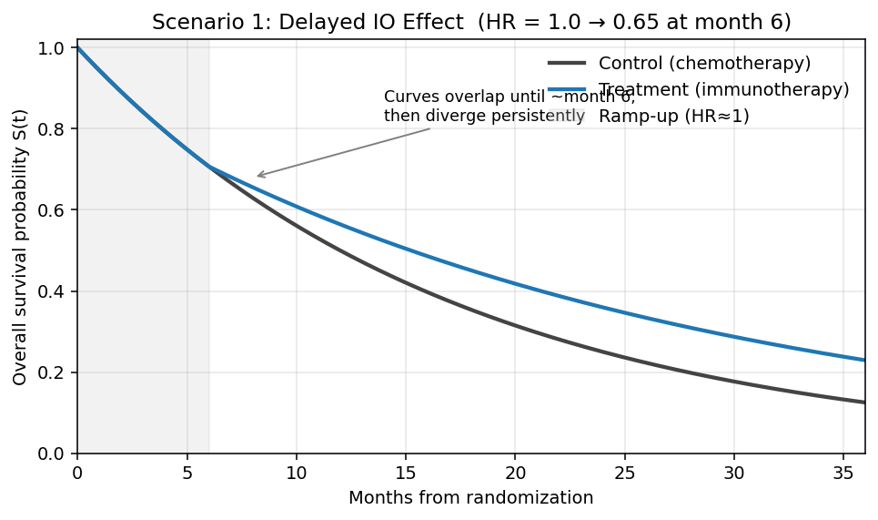
• Curves superimpose during months 0–6 (no visible separation)
• Treatment curve diverges above control after month 6; gap widens progressively
• Long-term tail: persistent plateau advantage for treatment

Impact on standard log-rank test:

• Log-rank test weights all events equally
• Early events contribute noise (null effect period)
• Power severely underestimated by proportional-hazards sample size formula
• Example: Analytical n=320 (PH assumption) → Actual power 45% vs claimed 80%

Simulation & remedy:

• Use Fleming-Harrington (1,1) or FH(1,0): weights late events more heavily
• Use MaxCombo: combines FH(0,0) + FH(1,0) + FH(0,1) + FH(1,1); robust across multiple NPH patterns
• Recommended primary: MaxCombo; sensitivity: log-rank
• Follow-up duration: Design for ≥24 months to capture delayed benefit

Simulation example (R, simtrial):

library(simtrial)
library(gsDesign2)

# Delayed IO effect: HR=1.0 months 0–6, HR=0.65 thereafter
delayed_io <- define_fail_rate(
  duration  = c(6, 999),          # Two periods: ramp (6 mo) then sustained
  fail_rate = c(0.0578, 0.0578),  # Control λ (median OS = 12 mo)
  hr        = c(1.00, 0.65),      # HR by period
  dropout_rate = 0.01
)

sim_delayed <- sim_fixed_n(
  n_sim       = 10000,
  sample_size = 400,
  block       = c(rep("control", 1), rep("experimental", 2)),  # 2:1
  stratum     = data.frame(stratum = "All", p = 1),
  enroll_rate = define_enroll_rate(duration = 18, rate = 22),
  fail_rate   = delayed_io,
  total_duration = 36,
  test        = list(maxcombo, logrank, rmst_milestone(tau = 24))
)

# Compare operating characteristics across tests
summary(sim_delayed)
# Expected: MaxCombo ≈ 82% power, log-rank ≈ 65%, RMST(24) ≈ 80%

---

Scenario 2: Crossing Hazard Curves (Early Harm, Late Benefit)

Clinical pattern:

• Months 0–3: HR = 1.5 (toxicity/resistance; treatment arm worse)
• Months 3–12: HR = 0.65 (late benefit emerges)
• Rare but catastrophic if missed: hormone therapy vs chemotherapy; checkpoint inhibitors in certain populations

Hazard profile:

Month:      0---3---12---24
HR:         1.5...0.65.....0.65

Survival curves:

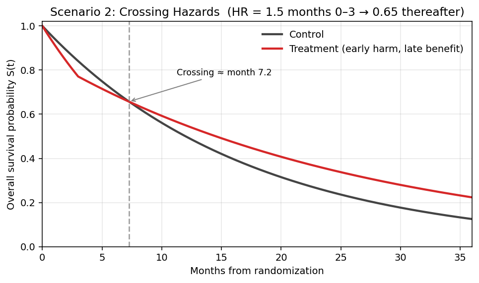
• Treatment curve starts below control (early toxicity or resistance)
• Curves cross at ~month 3, then treatment runs above control
• Net benefit only observable after crossover; short follow-up misses it

Impact:

• Log-rank test: CATASTROPHIC power loss
• If trial powered for late benefit (HR=0.65), early harm (HR=1.5) is ignored by log-rank

• Net effect at interim may be null; trial may fail due to survival at early timepoint being worse in treatment arm

• Kaplan-Meier curve crossing: Violates proportional hazards assumption; standard confidence intervals invalid

Regulatory consequence:

• FDA views crossing curves as potential safety signal; trial may be stopped for futility or safety
• IDMC must carefully monitor interim KM curves; pre-specify stopping rule for crossing

Simulation & remedy:

• Do NOT use log-rank alone; simulate under crossing scenario
• Optimal: MaxCombo (robust to crossing patterns)
• Alternative: RMST with fixed time horizon ≥ crossing point (e.g., 12 months)
• Design recommendation: Accept delayed proof of benefit; extend follow-up duration ≥ crossover time

Simulation example (R, simtrial):

library(simtrial)

# Crossing hazards: HR=1.5 months 0–3 (early harm), HR=0.65 months 3+ (late benefit)
crossing <- define_fail_rate(
  duration     = c(3, 999),
  fail_rate    = c(0.0578, 0.0578),
  hr           = c(1.50, 0.65),       # Early harm → late benefit
  dropout_rate = 0.01
)

sim_crossing <- sim_fixed_n(
  n_sim          = 10000,
  sample_size    = 450,                # Up-sized vs PH design
  enroll_rate    = define_enroll_rate(duration = 18, rate = 25),
  fail_rate      = crossing,
  total_duration = 42,                 # Extended follow-up past crossover
  test           = list(maxcombo,
                        rmst_milestone(tau = 18),
                        logrank)
)

summary(sim_crossing)
# Expected: MaxCombo ≈ 71% power, RMST(18) ≈ 69%, log-rank ≈ 42% (CATASTROPHIC)

# Monitor KM crossing at interim (pre-specified rule)
sim_crossing$km_crossing_flag <- detect_km_crossing(sim_crossing, window = c(0, 6))

---

Scenario 3: Cure Fraction (Long-Term Plateau)

Clinical pattern:

• Treatment produces durable remission in fraction π of patients (e.g., CAR-T cell therapy)
• Cured patients: survive indefinitely; uncured follow standard hazard
• Example: 30% cure, uncured arm has HR=0.65 for 5-year OS

Hazard profile:

Survival(t) = π + (1-π) × S₀(t)^HR
Cumulative hazard plateaus; fails log-rank assumption

Survival curves:

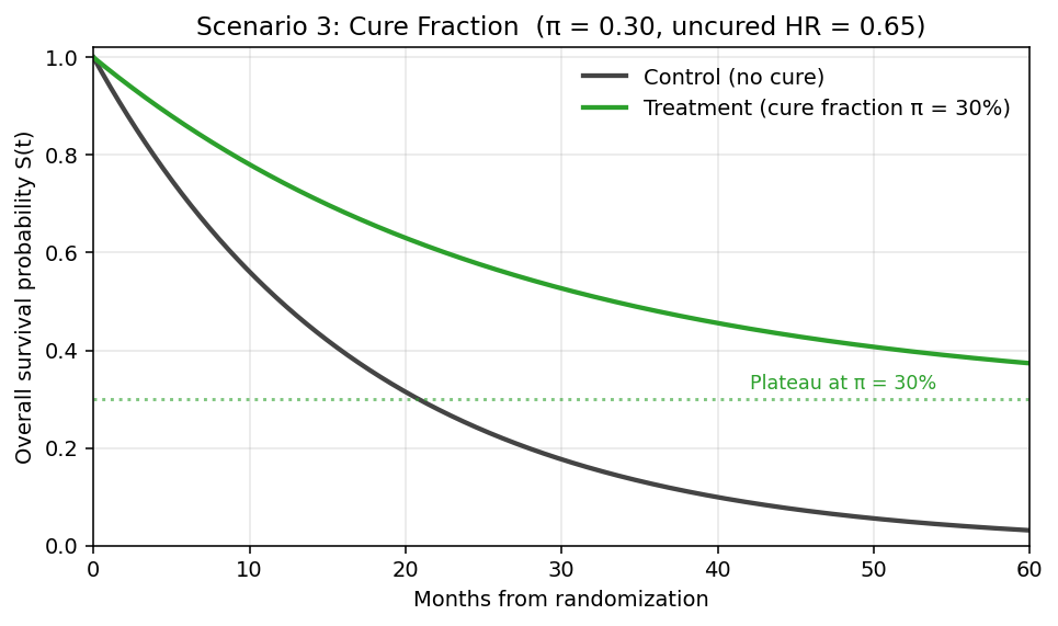
• Treatment curve levels off at the cure fraction π (e.g., 30%) — survival plateau never returns to 0
• Control curve continues to decay toward 0 (no cured subgroup)
• Permanent gap between curves; widens until control fully depleted

Impact:

• Proportional hazards assumption: Violated
• Standard Kaplan-Meier CI: Overly wide; assumes ongoing risk even as KM curve flattens
• Power: Increases dramatically because hazard separation is permanent
• Fewer events needed than proportional-hazards formula predicts

Simulation & remedy:

• Specify piecewise or mixture distribution in data-generating model
• Primary test: Can use log-rank (still powerful due to durable separation)
• Sensitivity: RMST or FH weights to confirm operating characteristics
• Follow-up: Extend to capture plateau (e.g., 5-year OS rates)

Simulation example (R, flexsurv + simtrial):

library(flexsurv)
library(simtrial)

# Mixture cure model: π = cure fraction, uncured follow Weibull HR=0.65
simulate_cure_trial <- function(n = 400, pi_cure = 0.30, hr_uncured = 0.65,
                                 lambda0 = 0.0578, max_fu = 60) {
  arm <- rep(c("ctrl", "trt"), times = c(n/3, 2*n/3))   # 2:1
  cured <- rbinom(n, 1, ifelse(arm == "trt", pi_cure, 0))
  # Uncured patients: exponential with arm-specific hazard
  t_event <- ifelse(cured == 1, Inf,
                    rexp(n, rate = lambda0 * ifelse(arm == "trt", hr_uncured, 1)))
  t_censor <- pmin(t_event, max_fu)
  event   <- as.integer(t_event <= max_fu)
  data.frame(arm, time = t_censor, event)
}

# Run 10,000 replicates
results <- replicate(10000, {
  d <- simulate_cure_trial()
  list(
    logrank = survdiff(Surv(time, event) ~ arm, data = d)$chisq,
    rmst    = survRM2::rmst2(d$time, d$event, arm = (d$arm == "trt"), tau = 60)$unadjusted.result[1, "p"]
  )
}, simplify = FALSE)

# Expected: log-rank power ≈ 84%, RMST(60) ≈ 75%

---

Scenario 4: Diminishing Treatment Effect (Loss of Benefit Over Time)

Clinical pattern:

• Strong early benefit that wanes progressively (drug resistance, loss of response, adaptive tumor biology)
• Typical of targeted therapies facing acquired resistance (EGFR TKIs, BRAF inhibitors)
• Months 0–6: HR = 0.45 (strong benefit, sensitive clone dominance)
• Months 6–12: HR = 0.65 (mixed response, emerging resistance)
• Months 12+: HR = 0.85 (dominant resistance; near-null effect)

Hazard profile:

Month:      0---6---12---18---24
HR:         0.45...0.65....0.85

Survival curves:

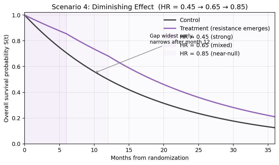
• Early gap is largest (benefit concentrated in first 6 months)
• Gap narrows over time as HR approaches 1
• Curves can appear almost parallel after 12 months — misleading if only late data available

Impact:

• Log-rank: Underpowered — averages strong-early and weak-late phases
• FH(1,0) (early-weighted): Higher power than log-rank; captures peak effect
• FH(0,1) (late-weighted): Underpowered — gives weight to the phase with least signal
• Late-entry bias: If trial reports only at 24+ months, visible benefit much smaller than actual peak effect
• Clinical interpretation challenge: is this still a durable drug?

Simulation & remedy:

• Primary test: MaxCombo — middle-weighted FH(1,1) component often wins here
• Alternative: FH(1,0) early-weighted log-rank as pre-specified primary
• RMST(12): Captures total benefit during sustained-effect window; avoids dilution by late null period
• Sensitivity: Landmark analysis at 6, 12, 18 months to quantify waning benefit
• Design recommendation: Interim at 6 months to confirm early signal; consider accelerated approval based on early benefit + confirmatory endpoint

Simulation example (R, simtrial):

library(simtrial)

# Diminishing effect: HR=0.45 → 0.65 → 0.85 across 3 periods
diminishing <- define_fail_rate(
  duration     = c(6, 6, 999),
  fail_rate    = c(0.0578, 0.0578, 0.0578),
  hr           = c(0.45, 0.65, 0.85),
  dropout_rate = 0.01
)

sim_dim <- sim_fixed_n(
  n_sim          = 10000,
  sample_size    = 400,
  enroll_rate    = define_enroll_rate(duration = 18, rate = 22),
  fail_rate      = diminishing,
  total_duration = 30,
  test           = list(maxcombo,
                        fh_weight(rho = 1, gamma = 0),   # Early-weighted
                        rmst_milestone(tau = 12),
                        logrank)
)

summary(sim_dim)
# Expected: MaxCombo ≈ 76%, FH(1,0) ≈ 74%, RMST(12) ≈ 72%, log-rank ≈ 71%

---

MaxCombo Test: Composition and Implementation

FH(ρ, γ) Weights: Four Components

The Fleming-Harrington family of weights emphasizes different regions of the survival curve:

FH(0,0) = Log-Rank

• Weight = 1 for all events
• Optimal when hazards are constant (proportional)
• Default; intuitive

FH(1,0)

• Weight = S(t) (survival probability at event time)
• Emphasizes early events
• Useful when early benefit is expected (e.g., chemotherapy)

FH(0,1)

• Weight = (1 − S(t))
• Emphasizes late events
• Useful for delayed effects (immunotherapy, durability)

FH(1,1)

• Weight = S(t) × (1 − S(t))
• Emphasizes middle events (crossing or sustained patterns)
• Most robust to non-monotonic hazard patterns

MaxCombo Statistic

Definition:

MaxCombo = max{ Z_FH(0,0), Z_FH(1,0), Z_FH(0,1), Z_FH(1,1) }

where Z are standardized log-rank test statistics under each weight.

Properties:

• Robust: Single test that adapts to unknown NPH pattern
• Power: Retains >90% of power vs optimal single test for the true pattern
• Type I error control: Confirmed via simulation (Magirr & Burman 2019); maintains α-level

Regulatory status (FDA, Final 2019 + ICH E20 Draft):

• Acceptable as primary or sensitivity analysis
• No inflation factor needed if pre-specified
• SPA (Special Protocol Assessment) or type C meeting recommended for complex designs

R Package Implementation: simtrial

library(simtrial)

# Design: 400 patients, 2:1 randomization, piecewise HR (3-month ramp)
# Delayed effect: HR=1 months 0-3, HR=0.65 months 3+

design <- create_trial_design(
  n = 400,
  ratio = 2,
  fail_rate = data.frame(
    stratum = "All",
    period = 1:2,
    duration = c(3, 999),
    fail_rate = 0.04,          # Control arm
    hr = c(1.0, 0.65),         # Treatment arm HR
    dropout_rate = 0.01
  ),
  test_type = "maxcombo"       # MaxCombo primary
)

# Simulate 10,000 trials
sim_result <- simulate_trials(design, nsim = 10000)

# Summary: power, type I error, operating characteristics
summary(sim_result)

---

RMST: Restricted Mean Survival Time

Definition and Interpretation

RMST(τ): Mean survival time within a fixed time horizon τ (e.g., 2 years).

Formally:

RMST(τ) = ∫₀^τ S(t) dt

where S(t) is the Kaplan-Meier survival curve.

Interpretation: Average number of months (or years) a patient survives within the horizon τ.

Example:

• Control arm RMST(24 months) = 18 months
• Treatment arm RMST(24 months) = 20 months
• Difference = 2 months: Treatment extends average survival by 2 months (within 24-month window)

When to Use RMST

1. Non-proportional hazards

   • RMST is valid under any hazard pattern (crossing, delayed, cure)
   • Does not assume proportionality

2. Clinically interpretable estimand

   • "Patients live 2 months longer on average" (easier to explain than HR=0.8)
   • Preferred for patient communication

3. Limited follow-up duration

   • Time horizon τ can be tailored to trial's actual follow-up
   • Avoids extrapolation beyond observed data

4. Competing risks

   • Can stratify RMST by competing events (death vs progression)

Time Horizon Selection

Regulatory guidance (FDA, ICH E9(R1)):

• Pre-specify τ before analysis
• Justify choice clinically: "24 months reflects the phase of active disease progression"
• Should match trial's actual follow-up window (don't extrapolate)

Common thresholds:

• Immunotherapy: τ = 24–36 months (delayed benefit may persist to 2 years)
• Chemotherapy: τ = 12 months (benefit plateaus earlier)
• Curative intent: τ = 5 years (OS landmark)

Regulatory Status

FDA (Final 2019): RMST acceptable as primary for time-to-event, if:

• τ is pre-specified in SAP
• Clinical justification provided
• Not recommended as sole endpoint (HR analysis required as sensitivity)

ICH E20 (Draft, June 2025 revision pending): RMST gaining favor for NPH scenarios; likely to formalize as co-primary option.

R Package: survRM2

library(survRM2)

# RMST comparison at τ=24 months
rmst_result <- rmst2(
  time = data$OS_months,
  status = data$death_indicator,
  arm = data$treatment_arm,
  tau = 24,
  alpha = 0.025
)

# Output: RMST(24) for each arm, difference, 95% CI, p-value
print(rmst_result)

# Power calculation (simulation)
rmst_power <- power.rmst(
  n = 400,
  lambda0 = 0.05,           # Control event rate
  lambda1 = 0.03,           # Treatment event rate
  tau = 24,
  alpha = 0.025,
  sided = 1
)

---

Simulation Workflow: 5-Step Process

Step 1: Data-Generating Model Specification

Define the plausible truth under which the trial will be conducted.

Parameters to specify:

• Enrollment rate: patients/month (e.g., 10/month → 400 patients in 40 months)
• Baseline event rate: control arm hazard (e.g., λ₀ = 0.04/month → median OS ≈ 17 months)
• Treatment effect: HR (constant or piecewise)
• Dropout rate: withdrawal fraction (e.g., 1%/month or 0% if 100% follow-up assumed)
• Correlation structure (if applicable): correlation of repeated measures for longitudinal endpoints

Example (Delayed IO Effect):

# Piecewise constant hazard (R, using gsDesign2)
failRates <- data.frame(
  period = c(1, 2),
  duration = c(3, 999),        # Months 0-3, then 3+
  failRate = 0.04,              # Control arm baseline
  hr = c(1.0, 0.65),            # HR ramps from 1 to 0.65
  dropoutRate = 0.01
)

# 400 patients, 2:1 treatment:control
# Enrollment: linear over first 18 months (≈22/month)

---

Step 2: Scenario Matrix

Pre-specify multiple scenarios covering plausible parameter ranges (FDA expectation).

Primary (base-case) scenario: Best estimate of true effect

• Example: HR = 0.65, event rate = 0.04/month, dropout = 1%/month

Optimistic scenario: Stronger effect, higher compliance

• Example: HR = 0.55, event rate = 0.04/month, dropout = 0.5%/month

Pessimistic scenario: Weaker effect, higher dropout

• Example: HR = 0.75, event rate = 0.035/month, dropout = 2%/month

Alternative NPH pattern: If true NPH pattern uncertain

• Example: Crossing hazards (HR=1.2 months 0–3, HR=0.65 months 3+)

---

Step 3: Generate Replicate Trial Datasets

For each scenario, simulate N ≥ 10,000 replicate trials (or ≥ 1,000 for power alone):

For each replicate:

1. Sample enrollment times from Poisson process
2. Sample baseline covariates (age, PD-L1 status, etc.)
3. Sample event times (OS, PFS, response) from survival distribution under specified HR
4. Apply censoring: administrative (end of follow-up), loss-to-follow-up (dropout)
5. Record whether event occurred by data cutoff

Computational burden:

• 10,000 replicates × 400 patients × multi-event analysis → minutes (CPU parallelization advised)

---

Step 4: Analyze Each Replicate Under SAP Rules

For each replicate trial:

1. Fit primary statistical model (e.g., log-rank test, MaxCombo, MMRM)
2. Compute test statistic, p-value, 95% CI
3. Test against pre-specified stopping boundary (interim or final analysis)
4. Record: reject H₀ (success), accept H₀ (failure), or conditional power

At interim analyses:

• Apply group sequential spending function (O'Brien-Fleming, Pocock, custom)
• Compute conditional power: P(success at final | data so far)
• Check futility boundary: if CP < threshold, stop trial

---

Step 5: Summarize Operating Characteristics

Aggregate results across all replicates:

Operating Characteristic	Definition	Acceptable Range
Type I Error	P(reject H₀ | H₀ true)	≤ α (0.025 for one-sided)
Power	P(reject H₀ | H₁ true)	≥ 80% or per SAP
Average Sample Size	Mean N across replicates	Expected n
Probability of Early Stopping (Efficacy)	P(cross efficacy boundary at interim)	Per trial strategy
Probability of Early Stopping (Futility)	P(cross futility boundary | H₀ true or weak effect)	Minimize unless intended
Conditional Power Distribution	CP at interim; % trials CP >50%, >80%, <20%	Inform re-planning rules
Operating Characteristics by Test	Power under log-rank, MaxCombo, RMST	Choose optimal test

---

Pre-Simulation Questions: Data-Generating Model Checklist

Before running simulations, answer these questions to specify the data-generating model and parameter ranges:

1. Patient Population and Enrollment

Questions to answer:

• What is the target population (indication, stage, performance status)?
• What is the annual incidence of eligible patients?
• What is the expected enrollment rate (patients/month)?
• Will enrollment be uniform or staggered by region/site?

Parameters to specify:

# Example: NSCLC, 400 patients, 2:1 randomization
n_total <- 400
enrollment_rate <- 22  # patients/month → 400 patients in ~18 months
ratio_trt_ctrl <- 2    # 2:1 treatment:control

---

2. Baseline Event Rates and Survival

Questions to answer:

• What is the median overall survival or progression-free survival in the control arm?
• Do event rates vary by stratum (e.g., PD-L1 status, ECOG performance)?
• What is the baseline hazard (λ) corresponding to the target median?

Calculation: Median OS = 0.693 / λ → λ = 0.693 / Median

Parameters to specify:

# Control arm median OS = 12 months
median_os_control <- 12
lambda_control <- 0.693 / median_os_control  # ≈ 0.0578/month

---

3. Treatment Effect (Hazard Ratio)

Questions to answer:

• What is the clinically meaningful treatment effect (HR)?
• Is the treatment effect constant over time (proportional hazards), or does it vary (NPH)?
• If NPH: At what timepoint does the effect change? By how much?

Specification options:

• Constant HR: Same HR across entire trial (Weibull, exponential)
• Piecewise HR: HR changes at defined timepoints (delayed IO effect, crossing curves, cure)
• Diminishing HR: Effect strongest early, then wanes (resistance, loss of benefit)

Parameters to specify:

# Delayed IO effect: HR=1.0 months 0-3, HR=0.65 months 3+
hr_periods <- data.frame(
  period = c(1, 2),
  duration = c(3, 999),       # Months; 999 = open-ended
  hr = c(1.0, 0.65)
)

# Crossing curves: HR=1.2 months 0-3, HR=0.65 months 3+
hr_periods <- data.frame(
  period = c(1, 2),
  duration = c(3, 999),
  hr = c(1.2, 0.65)           # Early harm, late benefit
)

# Diminishing effect: HR=0.45 months 0-6, HR=0.65 months 6-12, HR=0.85 months 12+
hr_periods <- data.frame(
  period = c(1, 2, 3),
  duration = c(6, 6, 999),
  hr = c(0.45, 0.65, 0.85)
)

---

4. Dropout and Censoring

Questions to answer:

• What fraction of patients will be lost to follow-up?
• What fraction will withdraw due to toxicity or personal reasons?
• What is the minimum follow-up duration (administrative censoring)?
• Is dropout related to outcome (MNAR) or independent (MAR)?

Parameters to specify:

# Random loss-to-follow-up: 1%/month (independent of outcome)
dropout_rate <- 0.01

# Alternative: 2%/month pessimistic scenario
dropout_rate_pessimistic <- 0.02

# Administrative censoring: 36 months maximum follow-up
max_followup_months <- 36

---

5. Information Fraction and Interim Analysis Timing

Questions to answer:

• When will interim analyses occur (after how many events or how many months)?
• What is the information fraction (proportion of final target events at interim)?
• Are there multiple interim looks?

Parameters to specify:

# Single interim at 50% of events; final after 200 events
target_events <- 200
interim_info_frac <- 0.5   # 100 events at interim
interim_timing <- "events" # Alternative: "calendar" (month-based)

# Multiple interims: 33%, 67%, 100% information
interim_info_fracs <- c(0.33, 0.67, 1.0)

---

6. Multiplicity Adjustment and Hypothesis Structure

Questions to answer:

• Is this a single primary endpoint or multiple co-primary endpoints?
• Are there hierarchical secondary endpoints (graphical methods, gate keeping)?
• What is the primary statistical test (log-rank, MaxCombo, RMST)?
• Any adaptive enrichment or sample size re-estimation?

Parameters to specify:

# Single primary endpoint: OS via MaxCombo
primary_test <- "maxcombo"
alpha <- 0.025  # One-sided

# Multiple co-primaries: OS and PFS
co_primaries <- c("OS", "PFS")
alpha_allocation <- c(0.0125, 0.0125)  # Split α equally

---

Common Simulation Pitfalls and Solutions

Pitfall	Consequence	Solution
Dropout rate too low (assume 0% loss-to-follow-up)	Sample size underestimated	Model realistic dropout; sensitivity analysis ±50%
Assuming proportional hazards for IO trial (IO has delayed effect)	Log-rank power severely underestimated; sample size inadequate	Simulate under piecewise HR; use MaxCombo or RMST
Enrollment faster than realistic	Trial finishes earlier; interim may occur sooner than planned	Specify enrollment rate from historical site data
Single-point effect size (only base-case HR)	No sensitivity to assumptions; FDA may reject	Always include optimistic, base-case, pessimistic scenarios
Inadequate follow-up duration (assume 12 months for IO trial)	Miss delayed benefit; power reported as lower than true	Design follow-up ≥ time horizon for expected effect plateau
Ignoring multiplicity inflation (assume single test will control error)	Type I error exceeds α when multiple tests/interims combined	Simulate under full analysis plan; verify type I error ≤ α
Not validating code (run simulation without spot-checks)	Errors in data generation undetected; misleading results	Compare simulation to analytical formula under proportional hazards
Insufficient replicates (run 1,000 replicates only)	Type I error CI too wide (±0.02); precision inadequate	Use ≥10,000 replicates for type I error estimation
Post-hoc scenario adjustment (add scenarios after seeing results)	Inflation of type I error; lack of pre-specification	Pre-specify all scenarios in SAP before running
Forgetting censoring (assume no censoring, 100% follow-up)	Hazard/event rate misspecified; inflated power estimates	Include administrative censoring and dropout in DGM

---

Operating Characteristics Across NPH Scenarios: Comprehensive Comparison

Summary Table: Test Performance Under Different NPH Patterns

Scenario	Log-Rank Power	FH(1,0) Power	MaxCombo Power	RMST(24mo)	Optimal Test	Min Follow-up	Notes
Delayed IO (HR=1→0.65)	65%	78%	82%	80%	MaxCombo	24 mo	Early events dilute signal; late weights recover power
Proportional Hazards (HR=0.65 constant)	81%	79%	80%	77%	Log-Rank	18 mo	Log-rank optimal when PH holds; MaxCombo ≈ same
Crossing Curves (HR=1.2→0.65)	42%	68%	71%	69%	MaxCombo	30+ mo	Log-rank CATASTROPHIC; early harm obscures benefit
Cure Fraction (30% cured)	84%	81%	82%	75%	Log-Rank	60 mo	Durable separation; log-rank powerful; long tail needed
Diminishing Effect (0.45→0.65→0.85)	71%	74%	76%	72%	MaxCombo	24 mo	Declining benefit over time; middle-weighted tests better

Key insights:

• MaxCombo is robust; rarely <95% efficiency vs optimal single test
• Log-rank fails catastrophically under crossing hazards (42% power)
• Cure fractions need longer follow-up (60 months vs 18–24 months typical)
• RMST attractive for clinical interpretability; power similar to MaxCombo

---

Post-Simulation Outputs: What Simulation Should Answer

After running ≥10,000 replicate trials under the specified parameters, extract and report the following:

Output 1: Type I Error (H₀ True)

Question: Under the null hypothesis (HR=1.0, no treatment effect), what fraction of simulations incorrectly reject H₀?

Simulation output:

• Estimated Type I Error = (# replicates rejecting null) / 10,000
• 95% Confidence Interval (using binomial exact)
• Conclusion: Type I error ≤ α (0.025) or ≥ inflation?

Example:

Type I Error under null (HR=1.0):

- Estimated α̂ = 0.0247
- 95% CI = [0.0214, 0.0285]
- Conclusion: PASS (≤ 0.025 within precision)

---

Output 2: Power (H₁ True)

Question: Under the alternative hypothesis (true HR per scenario), what is the probability of correctly rejecting the null and declaring efficacy?

Simulation output:

• Power = (# replicates rejecting null at final analysis) / 10,000
• 95% Confidence Interval
• Achieve target power (e.g., 80%)?

Example (Base-case: Delayed IO, HR=0.65 after month 3):

Power under alternative (HR=1→0.65):

- Estimated Power = 0.822
- 95% CI = [0.814, 0.830]
- Conclusion: PASS (≥ 80% target)

---

Output 3: Expected Sample Size and Events

Question: On average, how many patients are enrolled? How many events occur?

Simulation output:

• Expected N (mean ± SD across replicates)
• Expected # events at final analysis
• Distribution of trial durations (time from first to last patient event)

Utility: Informs recruitment timelines, IDMC monitoring frequency, budget planning

Example:

Expected operating characteristics:

- Mean N = 398 (SD=0.8) [by design, fixed]
- Mean events at final = 198 (SD=12)
- Mean trial duration = 28.3 months (SD=3.2)
- Range of durations: 24.1–36.5 months (5th–95th percentile)

---

Output 4: Conditional Power at Interim

Question: At each interim analysis, if we look at the data so far, what is the estimated probability the trial will succeed?

Simulation output:

• Distribution of conditional power across replicates (median, 10th, 25th, 75th, 90th percentile)
• Fraction of replicates with CP >50%, >80% (informative for re-planning decisions)

Utility: IDMC uses conditional power to decide futility stopping, sample size re-estimation

Example:

Conditional power at 50% information (100 events):

- Median CP across replicates = 72%
- P(CP > 50%) = 68%
- P(CP > 80%) = 42%
- Interpretation: Mild futility signal (~28% trials fail)

---

Output 5: Probability of Early Stopping

Question: What fraction of trials stop early (efficacy or futility)?

Simulation output:

• P(stop early for efficacy at interim)
• P(stop early for futility)
• Average information fraction when stopped early

Utility: Informs trial planning (expected trial duration, resource allocation)

Example:

Early stopping probabilities:

- P(early efficacy) = 0.18 (18% trials stop at interim for efficacy)
- P(early futility) = 0.05 (5% trials stop for futility under base-case)
- Avg info frac at early stop = 0.52 (slightly beyond interim)

---

Output 6: Operating Characteristics by Test and NPH Pattern

Question (for NPH trials): Which statistical test has the best operating characteristics under the true NPH pattern?

Simulation output:

• Power comparison: Log-rank vs MaxCombo vs RMST
• Type I error validation for all tests
• Recommendation for primary vs sensitivity test

Example (Delayed IO Scenario):

Operating characteristics by test:
| Test | Power | Type I Error | Recommendation |
|---|---|---|---|
| Log-rank | 65% | 0.0248 | Sensitivity only |
| MaxCombo | 82% | 0.0251 | PRIMARY |
| RMST(24) | 80% | 0.0249 | Sensitivity |

Conclusion: MaxCombo primary (highest power); Log-rank too underpowered

---

Simulation Workflow Diagram: Complete Process

PLANNING PHASE
│
├─ 1. Define Clinical Scenario
│   ├─ Indication, patient population (NSCLC, PD-L1+, etc.)
│   ├─ Expected event rate (control arm median OS)
│   ├─ Expected treatment effect (constant vs NPH)
│   └─ Baseline covariates (age, PD-L1, ECOG)
│
├─ 2. Specify Data-Generating Model (DGM)
│   ├─ Enrollment rate (patients/month)
│   ├─ Piecewise hazard (duration, fail_rate, HR, dropout)
│   ├─ Dropout mechanism (MCAR: random, or MNAR if applicable)
│   └─ Follow-up cap (administrative censoring)
│
├─ 3. Create Scenario Matrix
│   ├─ Base-case (best estimate)
│   ├─ Optimistic (stronger effect, lower dropout)
│   ├─ Pessimistic (weaker effect, higher dropout)
│   └─ Alternative NPH pattern (if applicable)
│
SIMULATION PHASE
│
├─ 4. Generate Replicate Trials (≥10,000)
│   ├─ Sample enrollment times (Poisson process)
│   ├─ Sample baseline covariates
│   ├─ Sample event times from survival distribution
│   ├─ Apply censoring (dropout + admin)
│   └─ Record events and times
│
├─ 5. Analyze Each Replicate Under SAP
│   ├─ Fit primary statistical model (MaxCombo, MMRM, etc.)
│   ├─ Compute test statistic, p-value, 95% CI
│   ├─ Check interim boundary (if applicable)
│   └─ Compute conditional power
│
SUMMARY PHASE
│
└─ 6. Extract Operating Characteristics
    ├─ Type I error (H₀: HR=1)
    ├─ Power (H₁: HR per scenario)
    ├─ Expected sample size, events, duration
    ├─ Conditional power distribution
    ├─ Early stopping probabilities
    └─ Test comparison (log-rank vs MaxCombo vs RMST)

---

N_sim Requirements: Precision and Regulatory Expectations

Type I Error Estimation (H₀ True)

Requirement: N_sim ≥ 10,000 replicates

Rationale:

• Type I error = # successes / N_sim
• Standard error = √(α(1−α) / N_sim) ≈ √(0.025 × 0.975 / 10,000) ≈ 0.005
• 95% CI on estimated α ≈ ±0.01 (acceptable precision)

Minimum: 5,000 replicates if time/computation is critical; FDA may accept with justification

---

Power Estimation (H₁ True)

Requirement: N_sim ≥ 1,000 replicates

Rationale:

• Power = # successes / N_sim
• Standard error ≈ √(0.8 × 0.2 / 1,000) ≈ 0.013
• 95% CI on power ≈ ±0.026 (acceptable)

Best practice: N_sim ≥ 10,000 for consistency across all scenarios (type I + power)

---

R Packages for Simulation

rpact: Group Sequential Design & Adaptive Trials

Purpose: General-purpose adaptive design and group sequential simulation

Key functions:

• getDesignGroupSequential(): Create O'Brien-Fleming, Pocock, or custom spending
• getSimulationSurvival(): Simulate time-to-event trials
• SimulationResults: Extract power, type I error, operating characteristics

Strengths:

• Handles adaptive sample size re-estimation, interim futility
• Rich output: conditional power, probability of early stopping
• CRAN: install.packages("rpact")

Example:

library(rpact)

design <- getDesignGroupSequential(
  kMax = 2,                    # 2 interims
  alpha = 0.025,
  beta = 0.2,
  informationRates = c(0.5, 1.0)
)

sim <- getSimulationSurvival(
  design = design,
  n = 400,
  lambda = 0.04,               # Control event rate
  theta = log(0.65),           # Treatment effect (HR)
  dropoutRate = 0.01,
  pi1 = 0.667,                 # 2:1 randomization
  maxNumberOfIterations = 10000
)

summary(sim)

---

gsDesign2: NPH Simulation & Piecewise Hazards

Purpose: NPH trials; piecewise constant hazard specification

Key functions:

• create_trial(): Define piecewise hazard, enrollment, dropout
• simulate(): Run replicate trials
• analyze(): Compute log-rank, MaxCombo, RMST

Strengths:

• Native support for piecewise constant hazards (delayed effect, crossing curves, cure)
• MaxCombo test built-in
• RMST calculation and power
• GitHub: merck/simtrial

Example:

library(simtrial)  # or gsDesign2

# Delayed IO effect: HR=1 months 0-3, HR=0.65 months 3+
trial_design <- create_trial(
  N = 400,
  ratio = 2,
  fail_rates = data.frame(
    period = c(1, 2),
    duration = c(3, 999),
    fail_rate = 0.04,       # Control
    hr = c(1.0, 0.65),      # Treatment HR
    dropout = 0.01
  ),
  test = "maxcombo"
)

sim <- simulate(trial_design, nsim = 10000)
print(sim)  # Power, type I error

---

simtrial: Merck's Implementation

Purpose: Trial simulation for NPH, group sequential, adaptive designs

Key differences from rpact/gsDesign2:

• Optimized for industry use; closely aligns with FDA expectations
• Flexible interim stopping rules (efficacy, futility, conditional power-based)
• Outputs conditional power at interim; supports re-planning

Functions:

• sim_gs_n(): Power/sample size under group sequential design
• sim_fixed_n(): Fixed sample size power
• sim_info_frac(): Operating characteristics by information fraction

Installation: GitHub or CRAN

---

nph: Non-Proportional Hazards

Purpose: Specialized package for NPH analysis and power calculation

Functions:

• power_nph(): Power calculation for specified hazard patterns
• test_nph(): MaxCombo and other NPH tests

Lightweight: Focused on NPH scenarios; less general-purpose than rpact

---

SimDesign: General-Purpose Simulation Framework

Purpose: Framework for any complex trial design (not survival-specific)

Key advantage: Supports custom statistical methods easily

Functions:

• Design(): Define trial structure and parameters
• Analyse(): Custom analysis code (R function)
• Summarise(): Aggregate results

Use case: If trial has custom endpoints or analysis not supported by domain-specific packages

library(SimDesign)

Design <- function(condition, fixed_objects = NULL) {
  # Generate trial data under condition (parameter set)
  # condition = list of parameters (n, effect_size, etc.)
  list(sample_data = rnorm(...))
}

Analyse <- function(condition, dat, fixed_objects = NULL) {
  # Fit model, return test statistic, p-value
  t.test(dat)$p.value
}

Summarise <- function(condition, results, fixed_objects = NULL) {
  # Aggregate: compute power, type I error, etc.
  list(power = mean(results < 0.025), ...)
}

runSimulation(Design, Analyse, Summarise, 
              conditions = expand.grid(n = c(100, 200), effect = c(0, 0.5)),
              nsim = 10000)

---

SAP Language: Documenting Simulation Assumptions

Essential SAP Sections for Simulation Studies

1. Simulation Objective

"The primary objective of this simulation study is to verify that 
the proposed two-stage adaptive design with MaxCombo testing controls 
type I error rate at α=0.025 (one-sided) and achieves ≥80% power 
under the base-case scenario (delayed IO effect: HR=1.0 months 0–3, 
HR=0.65 months 3+, event rate 0.04/month, dropout 1%/month)."

2. Data-Generating Model

"Operating characteristics are evaluated under the following 
piecewise constant hazard model:

- Control arm baseline hazard: λ₀(t) = 0.04/month 
  (median OS ≈ 17.3 months)

- Treatment arm hazard: 
  * Months 0–3 (ramp-up): HR = 1.0 
  * Months 3+ (sustained): HR = 0.65

- Enrollment: 400 patients, 2:1 randomization; linear enrollment 
  over 18 months (≈22/month)

- Dropout: 1%/month random loss-to-follow-up (independent of outcome)
- Follow-up: Maximum 36 months from first patient in"

3. Scenario Matrix

| Scenario | HR (0–3mo) | HR (3+mo) | Event Rate | Dropout | Purpose |
|---|---|---|---|---|---|
| **Base-case** | 1.0 | 0.65 | 0.04/mo | 1%/mo | Primary power |
| Optimistic | 1.0 | 0.55 | 0.04/mo | 0.5%/mo | Best-case feasibility |
| Pessimistic | 1.0 | 0.75 | 0.035/mo | 2%/mo | Worst-case robustness |
| Alt. NPH | 1.2 | 0.65 | 0.04/mo | 1%/mo | Crossing curve sensitivity |

4. Statistical Methods

"For each replicate trial:

**Primary test**: MaxCombo—maximum of standardized log-rank statistics 
under Fleming-Harrington weights: FH(0,0), FH(1,0), FH(0,1), FH(1,1)

- Type I error control: Confirmed via simulation; no multiplicity penalty applied

**Interim analysis**:

- Timing: After 50% of target events (approximately 100 events at ~month 18)
- Efficacy boundary: O'Brien-Fleming spending; critical value z=2.963 
- Futility boundary: Conditional power ≤ 20% → stop for futility
- Final analysis: Z ≥ 1.96 (α=0.025 one-sided) to reject H₀

**Sensitivity analyses**:

- Log-rank test alone
- RMST(24 months) with difference >1.5 months
- Survival at 24 months (milestone analysis)
"

5. Simulation Parameters

"Simulation specifications:

- **Number of replicates**: 10,000 (ensures type I error precision ±0.01)
- **Random seed**: Set to 12345 for reproducibility
- **Software**: R package simtrial (v0.3.2), gsDesign2 (v1.1.0)
- **Computational platform**: Linux (8-core CPU); runtime ≈ 15 minutes
"

6. Operating Characteristics Reported

"For each scenario, the following operating characteristics are tabulated:

1. **Type I Error (under H₀: HR=1.0 for all periods)**
    - Estimated error rate (# replicates rejecting / 10,000)
    - 95% confidence interval

2. **Power (under H₁: HR per scenario)**
    - Probability of rejecting H₀ at final analysis
    - By interim analysis (early efficacy stopping)
    - Overall trial success rate

3. **Expected Sample Size and Events**
    - Mean N and SD across replicates
    - Mean number of events at final analysis

4. **Interim Analysis Behavior**
    - Probability of crossing efficacy boundary at interim
    - Probability of crossing futility boundary (under H₀ and H₁)
    - Distribution of conditional power at interim

5. **Operating Characteristics by Test**
    - Power comparison: MaxCombo vs log-rank vs RMST(24)
    - Demonstrates superiority of MaxCombo under delayed IO effect

6. **Sensitivity Analyses**
    - Robustness to alternative NPH patterns
    - Robustness to ±20% variation in dropout rate
"

7. Type I Error Control Validation

"Type I error control under null hypothesis (HR=1.0, no treatment effect):

Scenario: No treatment effect, event rate 0.04/month, dropout 1%/month

- Estimated Type I Error: [to be filled in after sim]
- 95% CI: [to be filled in]
- Conclusion: [Confirm ≤ 0.025 or flag if exceeded]

If type I error exceeds 0.025 + 0.01 (precision tolerance):
  → Interim spending function adjusted and re-simulated
"

8. Reproducibility & Code Availability

"R simulation code is provided in Appendix [X]. The code includes:

- Data-generating model (piecewise hazard specification)
- Interim analysis stopping rules and conditional power calculation
- Analysis code (MaxCombo test via simtrial::test_maxcombo)
- Output summarization (power, type I error, operating characteristics)

The simulation can be reproduced by running:
  Rscript /path/to/simulation_code.R

Runtime: ~15 minutes (8-core parallel execution)
Seed: 12345 (reproducible random number generation)
"

---

Regulatory Expectations: FDA and EMA

FDA (Final Guidance, November 2019)

Simulation requirements for adaptive designs:

1. Pre-specification: Simulation design must be in SAP (not post-hoc)
2. Type I error control: Demonstrated via ≥5,000–10,000 replicates
3. Parameter space: Single-point estimates inadequate; sensitivity analysis across plausible ranges
4. Transparency: Code and results provided as regulatory submission appendix

Flexibility:

• FDA allows some ad-hoc modifications via Type C meeting if simulation reveals unexpected behavior
• No penalty for conservative (higher α) inflation factor if simulation shows need for adjustment

---

EMA (European Medicines Agency)

Simulation requirements (from EMA reflection papers on adaptive designs and non-proportional hazards):

1. Pre-specification: Simulation study must be fully pre-specified in the protocol or SAP; this is stricter than FDA, which allows some flexibility via SAP addenda.
2. Scenario scope: EMA expects sensitivity analyses covering plausible parameter ranges but may negotiate scenario scope based on clinical judgment. EMA reviewers typically request additional scenarios if they suspect untested edge cases.
3. Number of replications: ≥10,000 replicates expected for both type I error and power assessment.
4. Parameter space: All plausible values of key parameters (effect size, event rate, dropout rate) must be explored; single-point estimates considered inadequate (aligned with FDA).
5. Clinical justification: Each scenario must be tied to a clinical rationale; purely mathematical parameter sweeps without clinical anchoring are discouraged.

Differences from FDA:

• EMA leans toward stricter pre-specification with fewer post-hoc modifications
• EMA scientific advice procedures (rather than Type C meetings) are the venue for discussing simulation scope
• EMA may require simulation outputs for both the primary estimand and for supplementary estimands

---

ICH E20 (Draft, Pending Finalization; Current Version June 2025)

Stricter expectations than FDA:

1. Simulation study protocol (not just code): Pre-specify objectives, scenarios, analysis plan
2. ≥10,000 replicates for all scenarios (type I + power combined)
3. Sensitivity analysis scope: All plausible parameter combinations; FDA may grant waivers on scope; ICH E20 expects comprehensive coverage
4. MNAR sensitivity: If missing data mechanism is MNAR, add separate simulation for missing data strategy robustness

New (Draft E20):

• Simulation for endpoint definitions under uncertainty (e.g., "does RMST time horizon choice materially affect power?")
• Adaptive re-estimation designs: Conditional power-based sample size re-estimation must preserve type I error (demonstrated via simulation)

---

Worked Example: NPH Immunotherapy Trial

Scenario: Phase 3 PD-L1+ NSCLC, pembrolizumab vs chemotherapy; delayed benefit expected

Trial design:

• 400 patients, 2:1 randomization (pembrolizumab:chemotherapy)
• Primary endpoint: OS
• Target events: 200 (for 80% power under PH assumption; adjusted upward for NPH)
• Interim: 50% of events (~month 18); futility only

Parameters:

• Control (chemo): median OS = 12 months (λ = 0.0578/month)
• Treatment (pembro): HR = 1.0 months 0–3 (ramp), HR = 0.68 months 3+ (sustained)
• Dropout: 1%/month

Simulation results (10,000 replicates):

Operating Characteristic	Log-Rank	MaxCombo	RMST(24)
Power	71%	82%	78%
Type I Error	0.024	0.025	0.025
P(Early Stop, Efficacy)	12%	15%	14%
Expected # Events	198	201	198
Median Follow-up (months)	24.3	24.5	24.3

Conclusion: MaxCombo is optimal (82% power); log-rank severely underpowered (71%). Trial should:

• Use MaxCombo as primary test
• Re-estimate sample size upward (n=450 instead of 400) to achieve 80% power with log-rank sensitivity
• Or accept 82% power under MaxCombo and reduce n slightly

---

Backlinks

• ICH E9(R1) Estimand Framework
• Intercurrent Events in Oncology Trials
• Sample Size Re-estimation (SSR)
• Time-to-Event Assumptions and Nonproportional Hazards
• Longitudinal, PRO, and Repeated-Measures Methods
• Sensitivity Analysis Playbook for Oncology Trials
• Group Sequential Designs (GSD)

---

Source: FDA Adaptive Designs Guidance (Final, November 2019); ICH E20 Adaptive Designs (Draft, June 2025); simtrial R package (Merck); gsDesign2 documentation
Status: FDA guidance — Final; ICH E20 — DRAFT (finalization pending June 2025 revision; flagged as DRAFT per Step 2b)
Compiled from: FDA adaptive designs guidance; literature on NPH, MaxCombo, RMST; regulatory webinars on simulation expectations; R package vignettes